A6 – Fourier Transform Model of Image Formation

The Fourier Transform (FT) is a powerful algorithm used in signal and image processing that transforms a temporal signal to a frequency signal.

Familiarization with discrete FFT

Scilab has a function for 2 dimensional FT. This was explored and the results are shown in Figure 1.


Figure 1. (From left to right) Output for (a) intensity of fft, (b) shifted fft, (c) fft applied twice.

It is seen in Figure 1b that the output of the shifted FT of the circle matches the analytical FT of a circle which is an Airy pattern.


Figure 2. (From left to right) Output for (a) intensity of fft, (b) shifted fft, (c) fft applied twice.

The same procedure was done to a image of the letter A. It is seen that applying the fft twice results to an inverted version of the original image. This is because the result of fft2 has the quadrants along the diagonals interchanged.

Simulation of an imaging device

A digital camera has a lens with a finite size. This means that it could only gather a limited number of rays from the object resulting to a reconstruction that is not perfect. This phenomenon is illustrated here.


Figure 3. Original image simulating the object to be imaged.


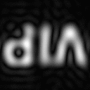
Figure 4. (From left to right) The "imaged" "VIP" for radii of increasing size.

The “imaged” “VIP” becomes closer to the original “VIP” with increasing radii of the white circle. This means that the larger the aperture of the lens, the higher the quality of the image.

Template Matching Using Correlation

Correlation measures the degree of similarity between two functions or images at that. The more similar they are at a certain position, the higher their correlation. This makes the correlation function very useful in template matching and pattern recognition.

Template matching is a pattern recognition technique used in identifying the common patterns in a scene such as a word or an image. This technique is applied to a text and the results are shown in Figure 5.


Figure 5. (From left to right) The first image is the text, the second is the letter "A" that we will find in the text, the third image shows the result after using the correlation function.

The result after using the correlation function is a map that lights up at the positions where we find the letter "A" in the text. Indeed we are able to find the identical patterns in this particular scene.

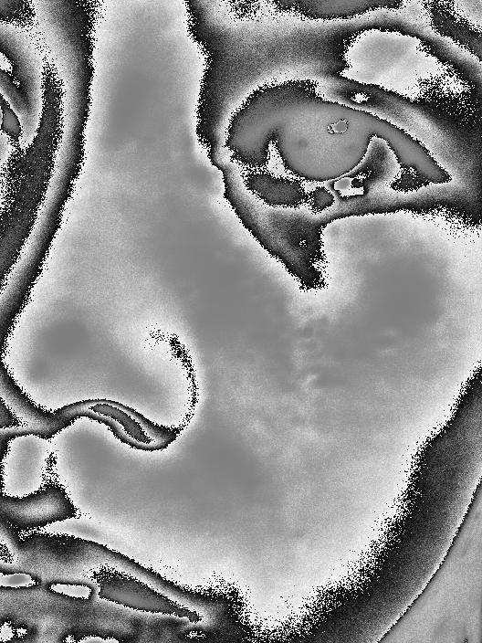
Edge detection using the convolution integral


Figure 6. (From left to right) Edge detection using a horizontal pattern, using a point pattern, and using a vertical pattern.

The convolved image for various patterns indicates the edges which are characterized by the pattern. The horizontal pattern makes all the horizontal edges light up, The point pattern makes the whole edge light up and the vertical pattern makes the vertical edges light up. Convolution is a very useful technique for edge detection.

For this activity, I give myself a grade of 10 because I implemented all the sub-activities and I learned and implemented various image processing techniques.

A5 - Enhancement by Histogram Manipulation

Histogram Equalization


Figure 1a ,1b, and 1c (from left to right)

Given a dark image with low contrast (Fig 1a), we could improve its equivalent grayscale image (Fig 1b) by manipulating its histogram, or the probability density function (PDF) of the different grayscale values of the image, shown in Fig 2a.

This is done using a simple process wherein we obtain the cumulative distribution function (CDF) shown in Fig 3a which is just the cumulative sum of the PDF (we use the function cumsum of Scilab). We create an 'ideal' CDF, which in this case is a straight increasing line for a uniform distribution. We then replace the dark pixel values with the intensity values from the desired CDF. To obtain faster calculations, we use the interp1 function of Scilab instead of using a for loop.

The histogram of the output image is shown in Fig 2b. We could see that it has a totally different shape from Fig 2a and shows a relatively uniform distribution for the different intensities. The histogram equalized image found in Fig 1c shows a brighter grayscale image than the original one (Fig 1b). Its cdf is shown in Figure 3b, showing a straight increasing line and verifying that our output follows the desired manipulation after processing the image.

Figure 2a and 2b (from left to right)

Figure 3a and 3b (from left to right)

Nonlinear Response


Figure 4a and 4b (from left to right)

The images above show the output images after using different nonlinear cdfs. Fig 4a is the output of a parabolic cdf (y = x^2). This image more closely models the response of the human eye in comparison to the histogram equalized image found in Fig 1c. Fig 4b shows a beautiful metallic image created using a cdf of the equation y = (x + 0.5)^-2. I also tried sine and cosine cdf's but they did not produce aesthetically pleasing results.

Using Advanced Image Processing Software (GIMP)



The histogram CDF could also be manipulated in GIMP as shown by the figure above. It is a cool application but I find it easier to define a cdf as in the previos procedure. This application of GiMP could be used for more personalized editing.

For this activity, I give myself a grade of 11 for discovering matrix calculations and trying out a wide range of different nonlinear cdf's to thoroughly explore this procedure.

A4 - Area Estimation for Images with Defined Edges

In this activity, the area of images with defined edges were obtained using two techniques: the Green's Theorem and morphological operations. Two types of shapes were considered. The first being a regular shape such as a circle or square whose area can be computed analytically, and the second, an arbitrary real shape such as the shape of the Dinagat Island found in Surigao del Norte obtained from Google Maps.

For the square, the area obtained using the Green's Theorem is 62001 pixels with 0.8 % error compared to the result using analytic and morphological operations which is 62500 pixels. For the circle, the area obtained using the Green's Theorem is 95319 pixels with 0.51 % error compared to the result using morphological operations which is 95812 pixels. The analytic area of the circle, 96211.275 pixels, varies from the actual area of the image (given by the result of morphological operations) because of the finite nature of the pixels.

For the shape of the Dinagat Island, the area obtained using the Green's Theorem is 32836 pixels with 2.49 % error compared to the result using morphological operations which is 33674 pixels. From the pixel to physical value conversion using the absolute scale of Google Maps and the value obtained using morphological operations, we compute the area to be 773.05 square kilometers with 3.62 % error compared to the recorded value of 802.12 square kilometers.

We find that the area obtained using the Green's Theorem exhibited less than 1 % error for the circle and square which are regular shapes and only 2.49 % error for an irregular shape such as an island compared to the actual area in the image obtained using morphological operations. Estimation of land area using these image processing methods as shown in the second example, gave 3.62 % error which could be attributed to the error in making the map, the difference in exposed land area due to tides, and the inclusion/exclusion of small islands surrounding the main island in the measurement of the recorded area.

For this activity, I give myself a grade of 11 for exploring two regular shapes which were the circle and the square, and for choosing a truly irregular shape such as an island to test the methods explored in this activity.

A3 - Image Types and Formats

Image Types

Binary Image

FileSize: 5135
Format: GIF
Width: 362
Height: 362
Depth: 8


StorageType: indexed
NumberOfColors: 256
ResolutionUnit: centimeter
XResolution: 72.000000
YResolution: 72.000000






Grayscale Image


FileSize: 77088
Format: JPEG
Width: 450
Height: 300
Depth: 8
StorageType: truecolor
NumberOfColors: 0
ResolutionUnit: inch
XResolution: 180.000000
YResolution: 180.000000

Truecolor Image

FileSize: 79400
Format: JPEG
Width: 563
Height: 422
Depth: 8
StorageType: truecolor
NumberOfColors: 0
ResolutionUnit: inch
XResolution: 72.000000
YResolution: 72.000000

Indexed Image


FileSize: 17324
Format: GIF
Width: 1024
Height: 768
Depth: 8
StorageType: indexed
NumberOfColors: 256
ResolutionUnit: centimeter
XResolution: 72.000000
YResolution: 72.000000

High Dynamic Range Image

FileSize: 588218
Format: JPEG
Width: 2048
Height: 1365
Depth: 8
StorageType: truecolor
NumberOfColors: 0
ResolutionUnit: inch
XResolution: 1.000000
YResolution: 1.000000

Multispectral Image

FileSize: 328466
Format: JPEG
Width: 1002
Height: 1002
Depth: 8
StorageType: truecolor
NumberOfColors: 0
ResolutionUnit: inch
XResolution: 72.000000
YResolution: 72.000000







3D Image (Stereopairs)

FileSize: 27220
Format: JPEG
Width: 448
Height: 336
Depth: 8
StorageType: truecolor
NumberOfColors: 0
ResolutionUnit: centimeter
XResolution: 72.000000
YResolution: 72.000000

Image Formats

TIFF or Tagged Image File Format is a lossless storage format for storing high quality digital images with the benefit of not incurring cumulative error when repeatedly editing and storing images. Its disadvantage is that it is not universally compatible, especially for web browsers, and the image size is much larger than other images compressed in different file formats.

JPG from Joint Photographic Experts Group is a universally compatible lossy storage format which can provide large compression of images with minimal loss in the quality perceived by our eyes. It is a good end format for transmission and archiving.

GIF or Graphics Exchange Format is limited to 256 colors and is generally "lossless" in storing images with colors less than this number, with large areas of the same color.

PNG or Portable Network Graphics stores images as indexed images like GIF, but is capable of storing 16 million colors giving it the capacity to store truecolor images. It is ideal for storing images with areas of uniform color and for displaying "lossless" images on the web.

BMP or Windows Bitmap is an uncompressed file format that handles graphics files for the Microsoft Windows OS.

RAW files are the original files stored in the digital camera that are not often compatible with other image editing or viewing software and are manufacturer dependent.

Other proprietary file formats of different image editing software like Photoshop or GIMP are ideal for storing works in progress but the final product is best to be saved as JPG or TIFF depending on the application.

Thresholding

The first figure at the left is the original image I used in Digital Scanning. The middle image is its histogram. Based on the histogram, I obtained the last figure by turning it to black and white with a threshold of 0.45. We can notice that in the third image, the grainy structures along the graph have disappeared.

For this activity, I would give myself a grade of 10 because though I posted it late, I still did my best. This activity also taught me a lot about the appropriate file formats to use for saving different images.