A13 - Color Image Segmentation

Color image segmentation has many applications in medical imaging, biomechanics, human and face recognition, remote sensing, and calculating percent cover in marine science. In this example, we want to segment the yellow of Haneka's dress. In my analysis, I used the Normalized Chromaticity Coordinates (NCC) so that the color is independent of the brightness information. The color segmentation itself can be done in two ways.

The first is the parametric method where the image is segmented using the joint probabilities of a pixel being in the region of interest using a Gaussian distribution and the mean and standard deviation of the pixel values in a cropped sample of the color of interest. The result is shown below.



The second is the non-parametric method where we get the 2D histogram of a cropped portion of the region of interest. We can see that the histogram is correct because it indicates a region in between the green and the red which corresponds to yellow.



I used this as a look up table for assigning values for the different pixels in the image. The results of histogram backprojection are shown below.



We can observe that the parametric method is more accurate in defining the region of interest based on the color than histogram backprojection. Histogram backprojection on the other hand is faster and more lenient because even reflections and other parts of an image light up. Histogram backprojection would still need a threshold to be accurate. On the other hand, the parametric method can be fairly stand alone.

For this activity, I give myself a grade of 15 for developing my own code for histogram backprojection far earlier than the start of this class.

A14 - Image Compression

Image compression is a useful way to enable the storing of large images in a small memory. The most popular file format for images, jpeg, also utilizes a compression technique in saving the images. The method that is shown here uses Principal Components Analysis and uses weighted basis images to represent blocks of the image.

The original image used is the sample image of Microsoft entitled Waterlilies.



I then got the grayscale image, cut the image into blocks and used PCA to get the eigenvectors that represent the basis images. I then examined the eigenvalues.

I then chose to use the first 20 eigenfunctions that would already provide 98.973403 % or about 99 % of the information of the image. Using these eigenfunctions, I got their coefficients by getting their dot products with blocks from the grayscale image. These coefficients are the weights of the different basis images used in reconstructing the block in the image. This is the code I used for reconstruction after getting the PCA of the blocks:

y = zeros(size(I));

k=0;

for r = 1:60
for c = 1:80
itemp = I(((10*r-9):(10*r)),((10*c-9):(10*c)));
xtemp = itemp(:);
k = c + (r-1)*8;
x(k,:) = xtemp';
for i = 1:20
atemp = sum(x(k, :)'.* facpr(:,i));
a(i) = atemp;
end
h = zeros(100,1);
for m = 1:20
ytemp = a(m)*facpr(:,m);
h = h + ytemp;
end
y(((10*r-9):(10*r)),((10*c-9):(10*c))) = matrix(h,10,10);
end
end

The reconstructed image is shown below.



Upon visual inspection, it contains all the information of the grayscale of the original image. It is observed that the 1 % loss in information is not evident and irrelevant in our application because we simply have to reconstruct the image and resolution is not of great importance. Therefore, our compression is successful for our purpose. It can also be computed that instead of saving 480,000 grayscale intensities for the 600 x 800 image, upon compression using the first 2o eigenvectors from the PCA, we only need to save 48,000 numbers instead because we only save 20 coefficients per 10 x 10 block. Theoretically, the file size is reduced to only 10 % of the original!

For this activity, I give myself a grade of 15 because I worked it out on my own and understood it well enough to teach it to a classmate.

A7 - Properties of the 2D Fourier Transform

The Fourier Theorem states that any signal or image can be represented by a superposition of sinusoids. Getting the Fourier Transform of a signal returns the spatial frequency distribution of the signal. In this activity, the rotation of the FT's upon rotation of the sinusoids was also observed.

Familiarization with FT of different 2D patterns

The image on the left is the object, the image on the right is the FT.

a. Square


b. Annulus


c. Square Annulus


d. Two slits along the x-axis


e. Two dots along the x-axis


Anamorphic pattern of the Fourier Transform

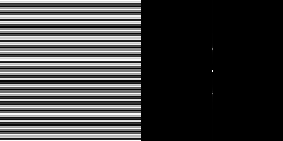
The following are sinusoids with increasing frequency. Their FT's are seen at the right

f = 4


f = 50


f = 100


We could observe that as the frequency increases, the dirac deltas that we see as dots move farther away from each other.

Adding a bias

Adding a constant bias:


Adding a constant bias shows a dot in the center representing that the constant has a zero frequency.

Adding a sinusoid with low frequency:


Adding a low frequency sinusoid as bias shows another pair nearer to the center in the FT.

Supposing that these images represent a real image of an interferogram in a Young's Double Slit experiment. We can get the actual frequencies by easy getting the Fourier Transform. Once this is done, we could now differentiate the bias and the signal. We could get the value of the actual frequencies by choosing the higher frequency and we could also reconstruct the signal by high pass filtering.

Rotating the sinusoid

theta = 30


Rotating the sinusoid results to an FT that is rotated also.

Combination of sinusoids in X and in Y



Combining sinusoids in X and Y result to an FT with dimensions along X and Y also.

Adding several rotated sinusoids



Even though the addition of different rotated sinusoids result to a chaotic signal, the FT is easily predicted by just adding the FTs of the individual sinusoids. I did this and I was able to correctly predict the FT of this noisy signal.

For this activity, I give myself a grade of 10 for understanding the basic properties of the Fourier transform.

A6 – Fourier Transform Model of Image Formation

The Fourier Transform (FT) is a powerful algorithm used in signal and image processing that transforms a temporal signal to a frequency signal.

Familiarization with discrete FFT

Scilab has a function for 2 dimensional FT. This was explored and the results are shown in Figure 1.


Figure 1. (From left to right) Output for (a) intensity of fft, (b) shifted fft, (c) fft applied twice.

It is seen in Figure 1b that the output of the shifted FT of the circle matches the analytical FT of a circle which is an Airy pattern.


Figure 2. (From left to right) Output for (a) intensity of fft, (b) shifted fft, (c) fft applied twice.

The same procedure was done to a image of the letter A. It is seen that applying the fft twice results to an inverted version of the original image. This is because the result of fft2 has the quadrants along the diagonals interchanged.

Simulation of an imaging device

A digital camera has a lens with a finite size. This means that it could only gather a limited number of rays from the object resulting to a reconstruction that is not perfect. This phenomenon is illustrated here.


Figure 3. Original image simulating the object to be imaged.


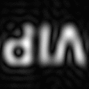
Figure 4. (From left to right) The "imaged" "VIP" for radii of increasing size.

The “imaged” “VIP” becomes closer to the original “VIP” with increasing radii of the white circle. This means that the larger the aperture of the lens, the higher the quality of the image.

Template Matching Using Correlation

Correlation measures the degree of similarity between two functions or images at that. The more similar they are at a certain position, the higher their correlation. This makes the correlation function very useful in template matching and pattern recognition.

Template matching is a pattern recognition technique used in identifying the common patterns in a scene such as a word or an image. This technique is applied to a text and the results are shown in Figure 5.


Figure 5. (From left to right) The first image is the text, the second is the letter "A" that we will find in the text, the third image shows the result after using the correlation function.

The result after using the correlation function is a map that lights up at the positions where we find the letter "A" in the text. Indeed we are able to find the identical patterns in this particular scene.

Edge detection using the convolution integral


Figure 6. (From left to right) Edge detection using a horizontal pattern, using a point pattern, and using a vertical pattern.

The convolved image for various patterns indicates the edges which are characterized by the pattern. The horizontal pattern makes all the horizontal edges light up, The point pattern makes the whole edge light up and the vertical pattern makes the vertical edges light up. Convolution is a very useful technique for edge detection.

For this activity, I give myself a grade of 10 because I implemented all the sub-activities and I learned and implemented various image processing techniques.

A5 - Enhancement by Histogram Manipulation

Histogram Equalization


Figure 1a ,1b, and 1c (from left to right)

Given a dark image with low contrast (Fig 1a), we could improve its equivalent grayscale image (Fig 1b) by manipulating its histogram, or the probability density function (PDF) of the different grayscale values of the image, shown in Fig 2a.

This is done using a simple process wherein we obtain the cumulative distribution function (CDF) shown in Fig 3a which is just the cumulative sum of the PDF (we use the function cumsum of Scilab). We create an 'ideal' CDF, which in this case is a straight increasing line for a uniform distribution. We then replace the dark pixel values with the intensity values from the desired CDF. To obtain faster calculations, we use the interp1 function of Scilab instead of using a for loop.

The histogram of the output image is shown in Fig 2b. We could see that it has a totally different shape from Fig 2a and shows a relatively uniform distribution for the different intensities. The histogram equalized image found in Fig 1c shows a brighter grayscale image than the original one (Fig 1b). Its cdf is shown in Figure 3b, showing a straight increasing line and verifying that our output follows the desired manipulation after processing the image.

Figure 2a and 2b (from left to right)

Figure 3a and 3b (from left to right)

Nonlinear Response


Figure 4a and 4b (from left to right)

The images above show the output images after using different nonlinear cdfs. Fig 4a is the output of a parabolic cdf (y = x^2). This image more closely models the response of the human eye in comparison to the histogram equalized image found in Fig 1c. Fig 4b shows a beautiful metallic image created using a cdf of the equation y = (x + 0.5)^-2. I also tried sine and cosine cdf's but they did not produce aesthetically pleasing results.

Using Advanced Image Processing Software (GIMP)



The histogram CDF could also be manipulated in GIMP as shown by the figure above. It is a cool application but I find it easier to define a cdf as in the previos procedure. This application of GiMP could be used for more personalized editing.

For this activity, I give myself a grade of 11 for discovering matrix calculations and trying out a wide range of different nonlinear cdf's to thoroughly explore this procedure.